Graph Neural Networks for Quine

Introduction

“Which records are the most similar to this one?”

That’s a straightforward question, but it hides some very thorny problems! Similar in what way? How do we measure similarity? How do we incorporate different attributes? How do we weigh different values? How do we incorporate similar relationships to other similar records?

Believe it or not, solving the similarity problem is more manageable than answering those questions. This is a perfect job for machine learning! New research in the last few years has brought natural language processing (NLP) tools to graphs as Graph Neural Networks (GNNs).

Graph A.I. is starting to leave the research lab and enable critical new use cases in the industry. From cybersecurity to fin-tech, to social networks, to ad placement, applications for graph A.I. are sweeping across industries.

While demonstrations on small datasets have proven the effectiveness and value of graph A.I. techniques, operationalizing graph A.I. in large graphs or with streaming data has been a significant obstacle!

The latest release of Quine includes built-in functionality for many of the essential graph A.I. algorithms. This changes with the 1.5 release of Quine. This post shows how to quickly solve tricky questions like “similarity” using Quine’s new random walk graph algorithm feature.

Take a Walk

Random walks are often the central connection between graph-structured data and machine learning applications. A random walk is a string of data produced by starting at a graph node, following one of its edges randomly to reach another node, then following one of its edges randomly to reach another node, and so on. Walks let us translate the possibly-infinite dimensions of graph data into linear strings we can feed to graph neural networks.

Generating one random walk in Quine 1.5 can be done by calling a function in a Cypher query:

MATCH (n) CALL random.walk(n, 10) YIELD walk RETURN id(n), walk LIMIT 1

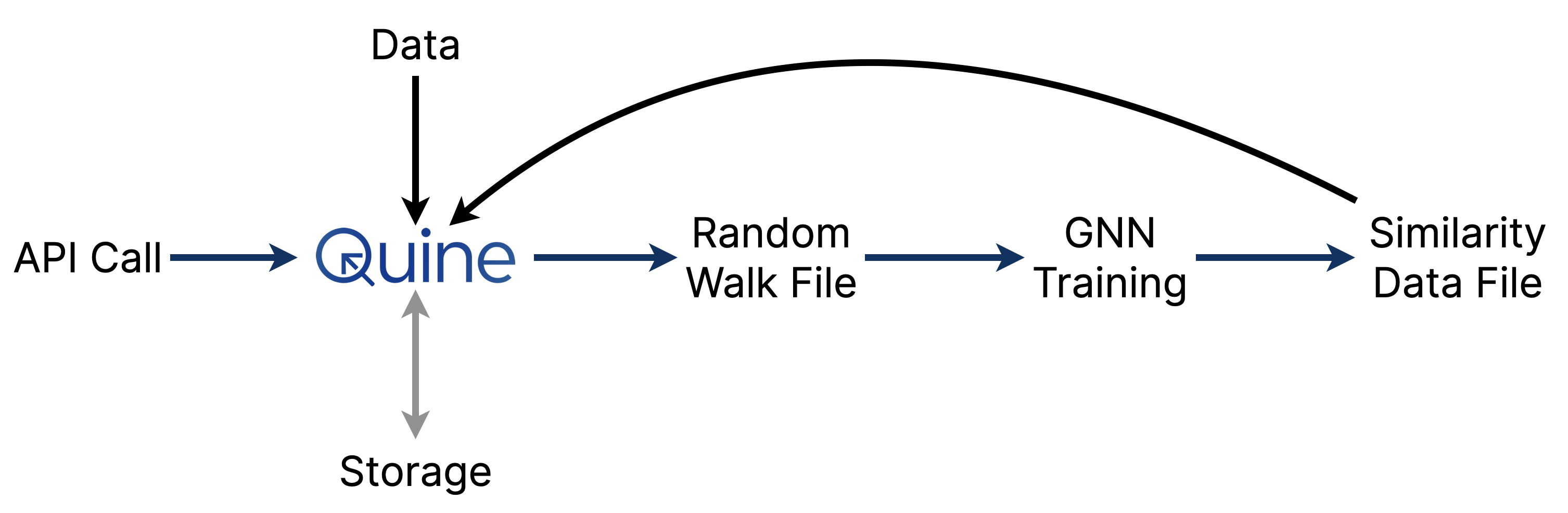
Or through an API call (if you know the ID of a node on which to start):

curl --request GET --url http://localhost:8080/api/v1/algorithm/walk/b93eabe7-38d2-30fa-8f96-097d75eb1f50

‍Take All the Walks

The previous examples start from one node and return one random walk. But graph A.I. usually requires building many walks from every node in the graph. To support this, Quine includes an API that will generate all random walks for an entire graph—regardless of how large the graph is.

Quine is a “streaming graph” that operates on continuous data streams. With an API call, you can direct Quine to stream all the random walks from every node in the graph to a file stored locally or in an S3 bucket.

curl --request PUT --url http://localhost:8080/api/v1/algorithm/walk --header "Content-Type: application/json" --data "{ 'bucketName': 'your-s3-bucket-name', 'type': 'S3Bucket' }"

‍Remember When

Most use cases for Quine include continuously-running data ingests that constantly modify the graph. To correctly generate a set of random walks, you need the graph to hold still while collecting random walk data. That’s hard to do in a stream that is constantly being updated with every new record that streams in.

Fortunately, it is straightforward to query a fixed graph in Quine using the historical query functionality. Include a historical timestamp with the at-time parameter in your query to generate random walks from the graph as it was at that fixed historical moment. **The rest of the graph can keep changing, but the GNN will see walks from a consistent and fixed view of the graph.**

curl --request PUT --url "http://localhost:8080/api/v1/algorithm/walk?at-time=$(date +%s000)" --header 'Content-Type: application/json' --data '{ "bucketName": "your-s3-bucket-name", "type": "S3Bucket" }'

Graph Neural Networks

Graph neural networks (GNNs) are a way to combine the power of graph-structured data and cutting edge machine learning techniques. Research on GNNs is continuing rapidly, but several foundational techniques have become critical to modern applications of artificial intelligence on graph data.

Node2Vec

The Node2Vec algorithm is a important technique for applying some revolutionary machine learning techniques to graph data. The initial Node2Vec paper by Grover and Leskovec appeared in 2016. It was an important paper which demonstrated how random walks on a graph behave like sentences in a corpus of natural language text. So by generating random walks, you could apply NLP (natural language processing) techniques and neural networks to graph data.

The NLP technique used by Node2Vec is Word2Vec. In 2013, Mikolov et. al published a landmark result showing that words from natural language can be “embedded” into a high-dimensional vector space. (Imagine plotting a point on a two-dimensional X-Y plane, but instead of 2 dimensions X and Y, put the dot in a plot with dozens, thousands, —or in the case of Large Language Models (LLMs)—hundreds of billions of dimensions!) The main take-away from this work is that word meanings can be learned by a computer and used mathematically. For instance, after training on English text, you can take the word “king”, subtract “man”, add “woman” and arrive at the word “queen”. Word2Vec works incredibly well for natural language; Node2Vec then took it a step further and applied this technique to graph data.

Random walks on a graph are the link that allows us to use Word2Vec for Node2Vec. A random walk generates a string of data from the graph. That string of data is analogous to a sentence in natural language. Producing many random walks gives us data structured like a set of documents containing many sentences; this is the “corpus” that trains the NLP model. So if we can produce random walks from a graph, we can train a neural network to learn the meaning of the data in that graph.

The random walk APIs in Quine 1.5+ allow a user to tune the random walks as described in the Node2Vec paper. The return parameter determines how likely a walk is to return one step back where it came from (to “backtrack” to the previous node). The in-out parameter determines whether a walk is more likely to explore the local region (“neighborhood”) around a node or travel far afield to explore corners of the graph far away. These parameters can tune the walks to learn different features of the graph and address different goals.

GraphSAGE

Whereas Node2Vec used random walks to generate a list of node IDs as the “corpus” to train Word2Vec, a richer approach was developed in the GraphSAGE algorithm. The primary development in GraphSAGE is to include the ability to explore the local area of each node in a walk, then aggregate features from each of the nearby nodes back to the starting node. These features then get concatenated together and used in the learning process for representing nodes in a graph. This provides two big improvements vs. Node2Vec: 1.) it provides a lot more information for each node (Node2Vec uses only the node’s ID), and 2.) it learns a function which can be used to embed unseen nodes—making it much more useful in practical situations where we need to compare new nodes not present in the original training set.

Embedding unseen nodes is important for streaming data workflows. It means that we can train a neural network on a consistent view of the graph at one moment in time, and then use that trained network to interpret new data (nodes) which stream in after the training. We can retrain the network any time we like, but we don’t have to skip over streaming data arriving in real-time. Every node can be embedded in real-time!

Quine’s random walk generation includes the ability to define an aggregation query for each node encountered in a random walk. This can be used to explore the local neighborhood and/or aggregate multiple properties which get automatically folded into the walk.

For example, the following Cypher query fragment is passed in to the query API parameter to collect different properties from nodes visited during a walk based on the node type:

RETURN CASE 
  WHEN "Movie" IN labels(thisNode) THEN thisNode.languages + [id(thisNode)] + thisNode.countries
  WHEN "Genre" IN labels(thisNode) THEN [id(thisNode), thisNode.genre]
  WHEN "Person" IN labels(thisNode) THEN [thisNode.born.year, id(thisNode), split(thisNode.bornIn, " ")[-1]]
  WHEN "Role" IN labels(thisNode) THEN id(thisNode)
  WHEN "User" IN labels(thisNode) THEN id(thisNode)
  WHEN "Rating" IN labels(thisNode) THEN thisNode.rating
  ELSE id(thisNode)
END

‍GNN Tutorial

Streaming data and graph neural network techniques come together in Quine 1.5 to easily solve some powerful graph A.I. use cases. Let’s use an existing recipe to demonstrate how we can enrich it with graph neural networks.

Let’s use the movieData recipe from here and enrich it using a GNN to compute similarity for movies in that dataset.

To get started, download the two data files to your working directory:
https://quine-recipe-public.s3.us-west-2.amazonaws.com/movieData.csv
‍https://quine-recipe-public.s3.us-west-2.amazonaws.com/ratingData.csv

Download the latest Quine executable.

Run the movieData recipe to ingest the movie data and build a graph:

java -jar quine-1.5.0.jar -r movieData --recipe-value movie_file=movieData.csv --recipe-value rating_file=ratingData.csv

Let that run to ingest all the data and build the movieData graph. When complete, you should see the ingest counters stop changing and an output that looks like this:

INGEST-4 status is completed and ingested 74090
INGEST-1 status is completed and ingested 74090
INGEST-2 status is completed and ingested 74090
INGEST-3 status is completed and ingested 74090
INGEST-5 status is completed and ingested 100005

We’ll use a Node2Vec approach for this example. Let’s start by generating random walks:

curl --request PUT --url "http://localhost:8080/api/v1/algorithm/walk?count=20&seed=foo&at-time=$(date +%s000)" --header 'Content-Type: application/json' --data '{ "type": "LocalFile" }'

NOTE: This bash command computes the current timestamp (in seconds) inline with date +%s and then appends 000 to make this a millisecond timestamp in the past.

This API call generates a string of node IDs by “walking” from every node in the graph, then saves a file to the local machine in the same working directory named something like: graph-walk-1674342158000-10x20-q0-1.0x1.0-foo.csv

NOTE: The file name is automatically derived from the parameters passed into the API call. If the API call includes a timestamp (in milliseconds), the filename will be the same if you issue the same API call again. If the API call includes at-time and a seed parameter, then the file contents will also be the same each time. But if the file already exists, trying to generate it again will return an error.

The first line of the file looks like this:

00006819-5fb1-310b-a4b6-e3bfbf600aa4,00006819-5fb1-310b-a4b6-e3bfbf600aa4,5f97b729-7435-3a44-823e-2e7217885d27,c9e28d23-5d1f-353a-b619-d1ec849d2583,c79ad95d-901d-3484-9f07-ae79c8efca39,ac799ac2-a21f-3b83-a827-31aace7c4211,c79ad95d-901d-3484-9f07-ae79c8efca39,0e415310-62ea-3bf6-b674-2ff5a9e84cee,985084e1-a9d5-353b-8080-175d2447929f,7a3c184f-451b-36ff-b005-feca7d8ee73b,985084e1-a9d5-353b-8080-175d2447929f,59cf0b79-23a1-36b8-96f6-ff6a4aa61e43

The line is a series of node IDs generated from a random walk starting at node 00006819-5fb1-310b-a4b6-e3bfbf600aa4.‍

NOTE: the first value of each line of the file output of the random walk call will always be the ID of the starting node, even if the walk returns other values. If a node has no edges to walk to, you’ll see a much shorter line: just the same node ID repeated twice.‍

The graph has 164,777 nodes. We instructed Quine to generate 20 random walks for each node. So the output file has 3,295,540 rows.

$ wc -l graph-walk-1674342158000-10x20-q0-1.0x1.0-foo.csv
 3295540 graph-walk-1674342158000-10x20-q0-1.0x1.0-foo.csv

‍Graph Embedding

With the random walks generated, we can use the output to train a neural network and load similarity data back into Quine (as a new ingest stream).

The following python code demonstrates how to train the neural net, create the embeddings, and computer similarity for each node in the graph:

Download This Code

import sys, json, requests
from gensim.models.word2vec import Word2Vec
from gensim.models.callbacks import CallbackAny2Vec
from multiprocessing import cpu_count
from datetime import datetime

file = sys.argv[1]

print(f"Reading in training data from: {file}")

line_count = 0
word_count = 0
data = []
with open(file, "r") as f:
	for line in f:
		l = line.strip().split(",")
		data.append(l)
		line_count += 1
		word_count += len(l)

print(f"Read in: {line_count} sentences with: {word_count} total words")

class EpochLogger(CallbackAny2Vec):
	'''Callback to log information about training'''
	def __init__(self):
		self.epoch = 1
	def on_epoch_begin(self, model):
		print(f"Iteration #{self.epoch} training started at: {datetime.now().strftime('%Y/%m/%d %H:%M:%S')}")
	def on_epoch_end(self, model):
		print(f"Iteration #{self.epoch} completed at: {datetime.now().strftime('%Y/%m/%d %H:%M:%S')}")
		self.epoch += 1
logger = EpochLogger()

print("Preparing dictionary and beginning model training...")
model = Word2Vec(data, vector_size=16, window=5, min_count=0, sg=1, workers=cpu_count(), callbacks=[logger])
print("Training Complete.")

ks = sorted(list(set([d[0] for d in data])))

print("Computing and saving similarities...")
with open(file + "-similarities.json", "w") as fd:
	for k in ks:
		d = { "target": k, "similarNodes": [{"id": x[0], "similarity": x[1]} for x in model.wv.most_similar(k)] }
		fd.write(json.dumps(d)+"\n")
print(f"Similarity save completed at: {datetime.now().strftime('%Y/%m/%d %H:%M:%S')}")

print("Saving the learned model...")
model.save(file + ".wvmodel")
print(f"Model save completed at: {datetime.now().strftime('%Y/%m/%d %H:%M:%S')}")

### Ingest similarities and create edges:
print(f"Beginning async ingest of similarity data from: {file}-similarities.json")
ingest_payload = {
  "type": "FileIngest",
  "path": file + "-similarities.json",
  "format": {
    "type": "CypherJson",
    "query": "UNWIND $that.similarNodes AS s MATCH (a), (b) WHERE id(a) = $that.target AND id(b) = s.id CREATE (a)-[:is_similar_to]->(b)"
  }
}
url = "http://localhost:8080/api/v1/ingest/similarities"
headers = {"Content-Type": "application/json"}
response = requests.request("POST", url, json=ingest_payload, headers=headers)
if response.status_code != 200:
	print(response.status_code)

Run this code with a command like (replace with your file name):

python graph_embedding.py graph-walk-1674342158000-10x20-q0-1.0x1.0-foo.csv

The script returns the following output from the training process:

Now we have similarity data saved to the file graph-walk-1674342158000-10x20-q0-1.0x1.0-foo.csv-similarities.json, which has single lines that pretty-print to look like this:

{
  "target": "00006819-5fb1-310b-a4b6-e3bfbf600aa4",
  "similarNodes": [
    {
      "id": "b221ceb5-9a0a-3c93-b0d0-870ab56ff924",
      "similarity": 0.9671398997306824
    },
    {
      "id": "97290657-1a1e-34c1-8bd1-3db0aefaf13b",
      "similarity": 0.957493245601654
    },
    {
      "id": "2fa7e55a-840e-37ec-bb30-8736e71d037b",
      "similarity": 0.9573205709457397
    },
    ...
  ]
}

The data in this file tells us that, for each target node, we have a measure of its similarity to the other node somewhere else in the graph with the corresponding id. We’ve saved the top-10-most-similar-node-ids for each node in the graph to a file.

Each pair of target and similarNodes.id generated in the ...similarities.json file is a new edge we can create and name is_similar_to.

After saving the learned model, our Python script made an API call creating an ingest stream named similarities to load the data into Quine. Once it’s complete we can visualize the data.

Check the status of the similarities ingest stream with an API call like:

curl --request GET --url http://localhost:8080/api/v1/ingest/similarities

{
  "name": "similarities",
  "status": "Completed",
  ...

‍Seeing Similarities

Our graph now has edges showing the results for the question we began with:

“Which records are the most similar to this one?”

Let’s see which movies are similar to each other:

MATCH (n: Movie)-[:is_similar_to]->(m: Movie)-[:is_similar_to]->(n) RETURN n, m LIMIT 100

And we get insightful results:

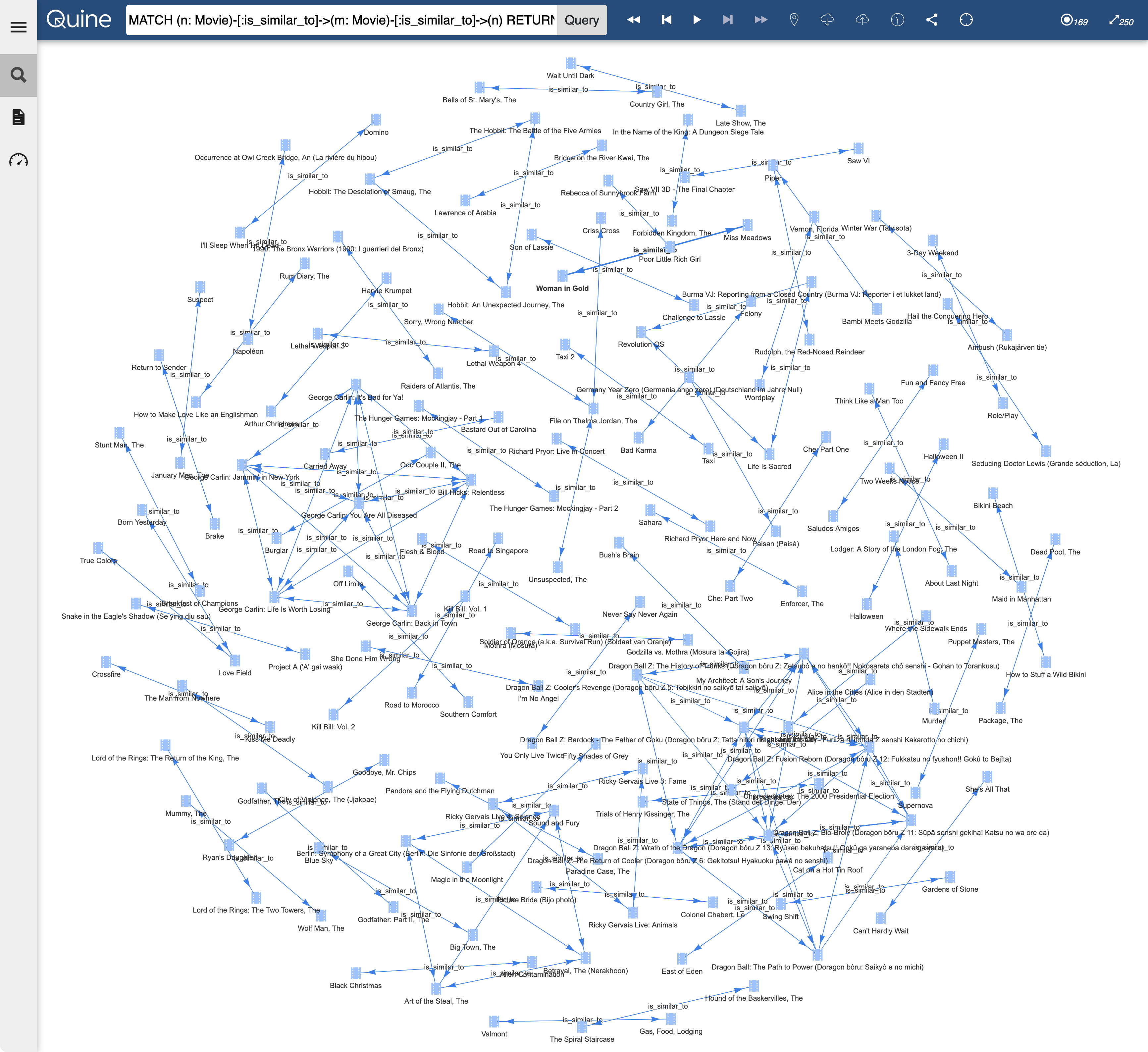
This graph is a lot of fun to explore! Looking at a few of the connections, we see that the GNN learned many useful similarities:

• The Hobbit trilogy appears in a connected triangle near the top.
• The George Carlin (and Bill Hicks) pentagram is left of center.
• Many sequels are related to their predecessors.
• A pair of Bond movies appears just below the center (more if we didn’t limit results)
• Movies in the same genre are much more likely to be similar.
• …and many more! Your version might be a little different based on the randomness of the GNN training. Take a look and see what you find.

Similar movies will have similar genres, similar actors in similar roles, similar users providing similar ratings, similarities of similarities, and so on. The similarities also include the dataset’s other kinds of graph relationships. The entire graph is incorporated into the graph neural network learning process through random walk production.

Want to explore more kinds of similarities? Try this query to explore similar actors:

MATCH (n: Person)-[:is_similar_to]->(m: Person)-[:is_similar_to]->(n) RETURN n, m LIMIT 100

‍Conclusion

Machine Learning on graphs is an effective new technique applicable to all sorts of datasets—even many that don’t immediately need a graph. Representing JSON or CSV data as a graph allows us to draw connections that become crucial for neural networks to draw conclusions that would otherwise be impossible to detect or require enormous manual human analysis.

This is only the beginning! In a future post, we’ll look at how to apply these graph neural network techniques to your live streaming data to constantly embed new nodes which weren’t part of the training set.